|
|
Movies:
- I started doing SLAM in 2002 on a robot called Pluto. Here is what Pluto looks like: Pluto
in
the
bakery.
- Here is Pluto making a large outdoor map using a
Compressed
Extended
Kalman
Filter back in 2002: Compressed
Kalman
Filter. The robot is the small x. The map is a
surveyed map of the buildings and very accurate. The walls are
detected by a SICK laser scanner and formed into a map. Each new
measurement is used to improve the map and the location of the small
x.
- I improved the estimate of the maps and location by
developing a graphical SLAM method. This was amoung the first to sucessfully close a loop in a large map. Here is an example of
using Graphical (Robust) SLAM
to close a
large
loop, avi: Graphical
Slam With Loop Closing . The dots being left behind the robot
as it
moves are additional states being estimated. Having these
additional states allows better linearization of the system.
It also creates a sparse structure of connections between
the features that can be exploited to speed the calculations.
After this work was done there was a wave of interest in sparse SLAM
methods.
- Patric Jensfelt and I demonstrated one of the first camera based SLAM systems in 2005. Here is a movie showing a robot mapping our lab
using a
camera
(slowed down to half actual speed of the offline calculation) EKF
SLAM using Vision and M Space. This uses a
standard SLAM but using a camera to do SLAM with constraind 3D lines is
tricky. We developed a way to represent the constraints on the
lines so that they could be used as 1 or 3 dimensional features.
- Here is a movie showing a map of our lab using a camera and
SICK
scanner, EKF
SLAM using Vision, SICK, and M Space. Using different types
of sensors presents a challenge in fusing the information from the
sensors that can be qualitatively different.
- Here is a movie showing a graphical map of our lab using a
camera, Graphical
SLAM using Vision and M Space.
- Here is another movie showing a graphical map of our
lab using a
camera where we merge star nodes to build constraints into the
graph, Graphical
SLAM using Vision and
M Space.
- Here is a movie showing a graphical map
of our old
lab. Here we detect 3 separate loops automatically and
enforce the constraint on the graph. Closing
the Loop Automatically with Graphical SLAM.
- Something completely different, the Antiparticle filter. Compared to the Particle filter. Here we simulate how very noisy odometry can be corrected with proper correllations in an adaptive analytic recursive Baysian filter.
-
Moving
Underwater
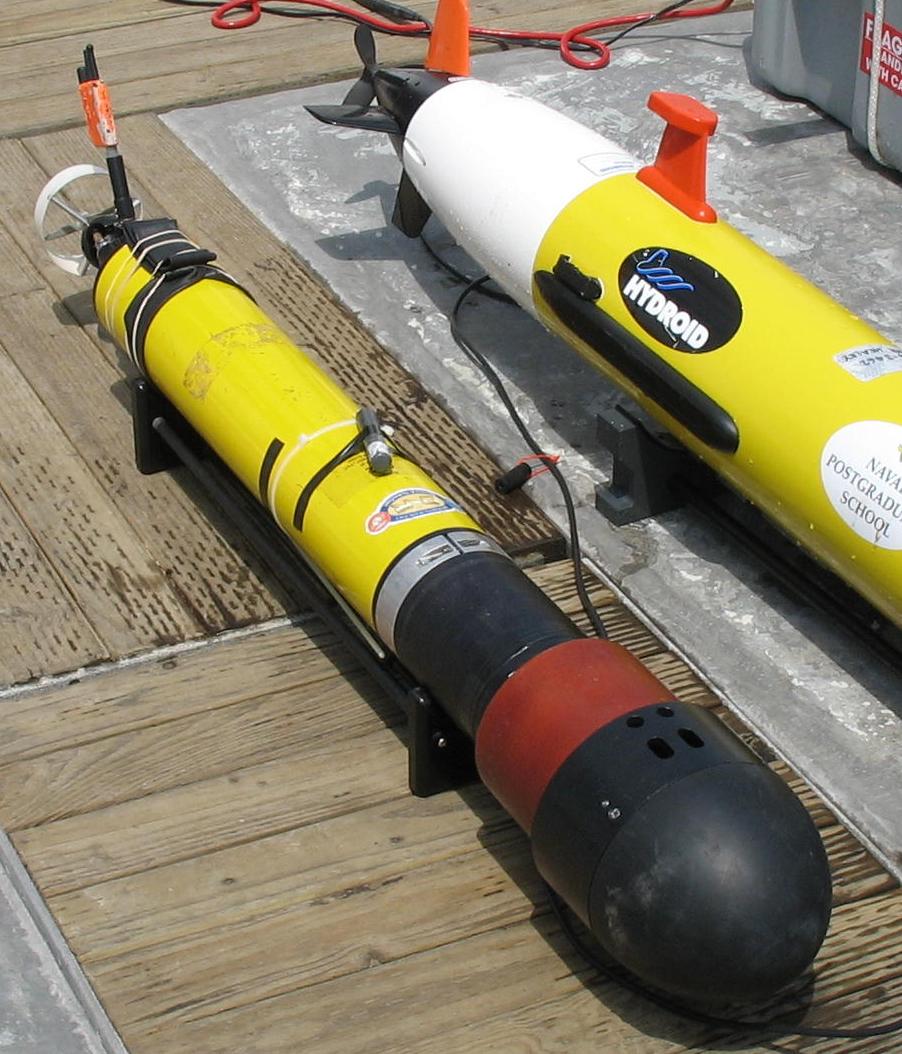
- Here is a movie showing an autonomous underwater
vehicle, AUV,
matching a SLAM map to an a
priori map: Underwater
SLAM. This is a complete navigation system. It includes
5 estimators: 3 EKF's, a prediction filter, and a tracking
filter. The tracking filter uses a novel feature representaion
and a graphical SLAM algorithm to make sense of sonar and motion
data. It passes what it learns as chunks of information on entire
local areas to a global EKF. This happens at a slow rate (every
15-100 seconds). The global estimator can then match to the a
priori map. This system has since developed into a very
robust navigation system that can handle large amounts of ambiguity
(see below). It is fast enough to be used for control, (and we do
that).
- Here is another movie showing the AUV
matching a SLAM map to the a priori map. The correct
matching is chosen at last but the robot chooses some more aggressive
hypothesis first. Then, as more information comes in, it switches
to a more likely conservative matching hypothesis: Multihypothesis
Matching. Here is a
simple matching that looks to a human like it works but not if you look
at the first movie; this was the live result: Almost
Right.
- We went back and re-thought things and two months later...
Here we have a perfect day of testing. A rare event
in robotics. The goal here is to have the AUV find the designated
target (the circled star in the middle of things). The robot must
match the confusing sonar pings in light
blue with the approximate a priori map, the tiny purple
dots. The double rings are matched features: Five
for Five. This uses a new matching metric that we plan
on publishing a paper on soon. Here is a longer look at the forth
run that day Run4.
- We have since added an attachement mechanism to the robot
and done ocean trials with high success rates in attaching to the
chosen target. Here the
moored target is at 20 feet altitude and the last in the third
line. The robot uses the bottom features to navigate to the
target then increases its altitude before attaching to the line.
|
|
Contact
details
|
John
Folkesson.
RPL, EECS, KTHy
Kungl
Tekniska
Högskolan
SE-100
44 Stockholm
Sweden
|
|