weinkauf/notes/reconstruct1d

Topology-based Smoothing of 1D Functions

Reconstruct1D is a tool for smoothing one-dimensional data based on topological constraints. Consider some input data containing a number of local minima and maxima. Given a selected subset of these minima/maxima, Reconstruct1D will produce a smoothed version of the input data with the following properties:

• the output data contains only the selected subset of minima/maxima,
• the output data is smooth in the sense of C1 or C2 continuity (user parameter),
• the output data is as close as desired to the original data (user parameter).

When working with noisy input data, the tool is best paired with Persistence1D: a tool for extracting and filtering extrema of one-dimensional data. The tool can just as well be used to create smooth one-dimensional data with topological constraints from scratch as can be seen in an example below.

The package supports Python and Matlab.

The Matlab version of Reconstruct1D has been written by Yeara Kozlov and Tino Weinkauf, Max Planck Institute for Informatics, Saarbrücken, Germany. The Python version has been written by Tino Weinkauf, KTH Royal Institute of Technology, Stockholm, Sweden. You may use the code as you wish, it is in the public domain. If you find it useful, it would be nice to hear from you. Just drop us a line.

Reconstructing a smoothed version of the input function that contains only the filtered set of extrema.

Overview

The algorithm is available in Python and Matlab:

• Python: This is a re-implementation of the older Matlab code. It is cleaner and more documented. Only a single import statement is required. The code depends on the Python packages numpy and qpsolvers. The latter provides a unified API to a larger number of Quadratic Programming solvers (e.g., quadprog, cvxpy, ecos, and others) of which at least one has to be available. Reconstruct1D assumes quadprog to be available by default. These dependencies can be quickly installed using pip:

  • pip install numpy
  • pip install qpsolvers
  • pip install quadprog

• Matlab: the code can be used from within Matlab straightforwardly. The use of MOSEK can be enabled to achieve fast computation times.

Both version should be used in conjunction with their respective Python/Matlab Persistence1D counterpart.

Example for Python

A simple function call suffices to get the smoothed data with as many sample points as were given in the original data. All code is located in the python folder.

import matplotlib.pyplot as plt
import numpy as np
from persistence1d import RunPersistence
from reconstruct1d import RunReconstruction

#~ Generate data using sine function and different frequencies.
x = np.arange(600.0)
SineLowFreq = np.sin(x * 0.01 * np.pi)
SineMedFreq = 0.25 * np.sin(x * 0.01 * np.pi * 4.9)
SineHighFreq = 0.15 * np.sin(x * 0.01 * np.pi * 12.1)
InputData = SineLowFreq + SineMedFreq + SineHighFreq

#~ Compute the extrema of the given data and their persistence.
ExtremaAndPersistence = RunPersistence(InputData)

#~ Keep only those extrema with a persistence larger than 0.5.
FilteredIndices = [t[0] for t in ExtremaAndPersistence if t[1] > 0.5]

#~ This simple call is all you need to reconstruct a smooth function containing only the filtered extrema
SmoothData = RunReconstruction(InputData, FilteredIndices, 'biharmonic', 0.0000001)

#~ Plot original and smoothed data
fig, ax = plt.subplots()
ax.plot(range(0, len(InputData)), InputData, label="Original Data")
ax.plot(range(0, len(SmoothData)), SmoothData, label="Smooth Data")
ExtremaIndices = [t[0] for t in ExtremaAndPersistence]
ax.plot(ExtremaIndices, InputData[ExtremaIndices], marker='.', linestyle='')
ax.plot(FilteredIndices, InputData[FilteredIndices], marker='*', linestyle='')
ax.set(xlabel='data index', ylabel='data value')
ax.set_aspect(1.0/ax.get_data_ratio()*0.2)
ax.grid()
plt.legend()
plt.show()

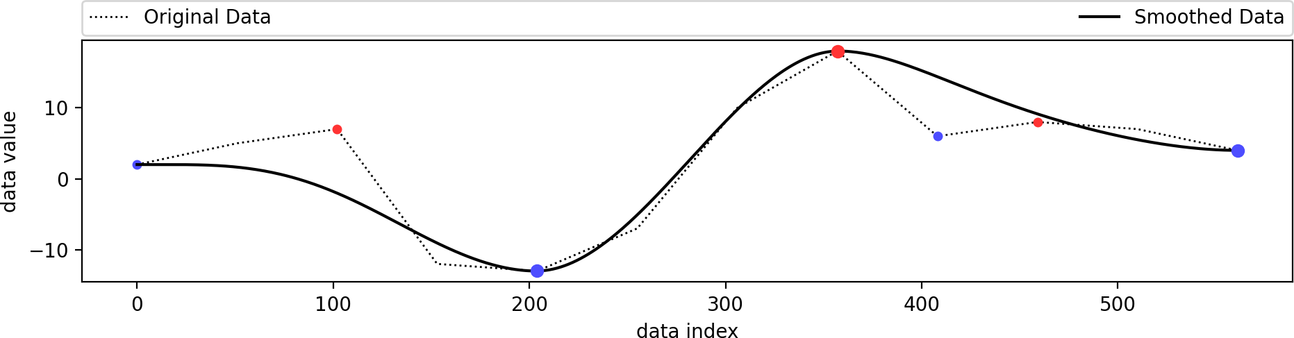
Running the code from above yields this output:

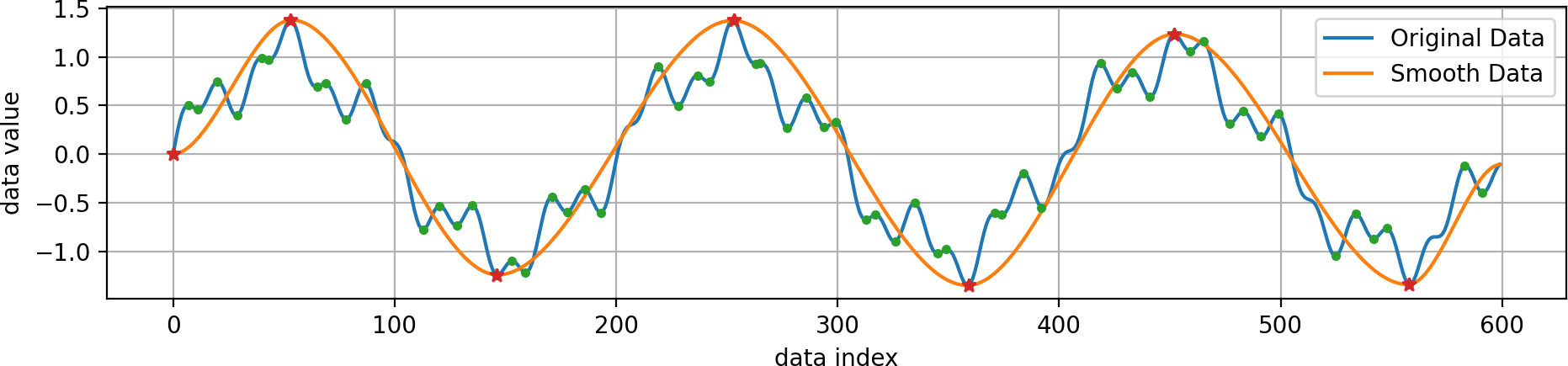
The original data (blue) is a combination of several sine functions with different frequencies. Its minima and maxima are shown as green dots, of which only a few have been selected to remain (red stars), since they have a higher persistence. The smoothed data (orange) containes only these selected extrema and follows the original data in a smooth manner.

More Examples

The code for the following examples can be found in the file examples_reconstruct1d.py in the python folder.

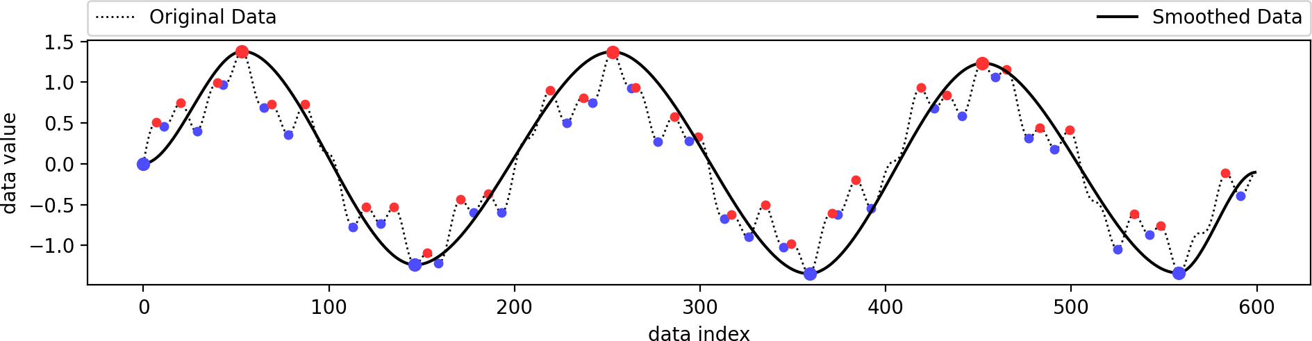
This is identical to the example from above. We just use a better visualization setting here. The original data is a combination of several sine functions with different frequencies. Its minima (blue) and maxima (red) are shown as dots, of which only a few have been selected to remain (larger dots), since they have a higher persistence. The smoothed data containes only these selected extrema and follows the original data in a smooth manner.

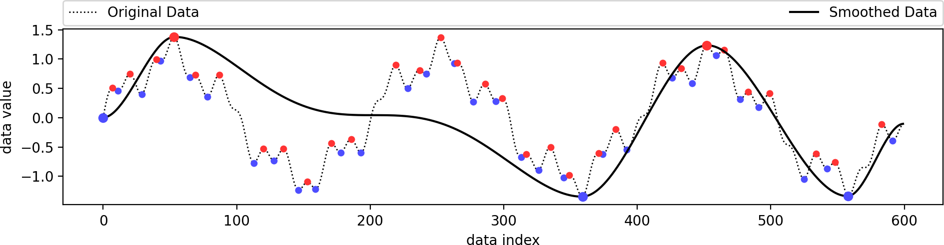
We manually filtered out a minimum/maximum pair from the previous example and reconstructed a smooth function based on the remaining extrema. As long as the set of selected extrema is topologically consistent, the output is guaranteed to contain only these extrema.

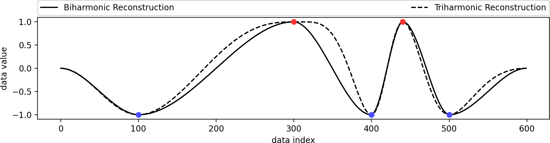
We created a set of extrema from scratch and reconstructed a biharmonic and triharmonic function from these topological constraints only. This can be useful in certain scenarios where users shall be able to create and manipulate functions. This example also serves the purpose of highlighting the difference between a biharmonic and a triharmonic reconstruction. A biharmonic reconstruction yields a C1 continuous curve: its first derivative (tangent vector) is continuous. A triharmonic reconstruction goes one step further and yields a C2 continuous curve: its first derivative (tangent vector) is smooth. While this sounds desirable, it also creates some potentially unwelcome behavior. The suggestion is to go with a biharmonic reconstruction for most cases.

This example shows the influence of the data weight parameter. A value of zero ignores the shape of the original data and just interpolates the given extrema in a biharmonic or triharmonic manner. Values larger than zero follow the shape of the original data more closely.

Smoothness requires a reasonable level of sampling resolution. Our code does not change the resolution by itself, but it is trivial to provide a linearly supersampled version of the input data, which leads to a very smooth final result. In this example, the input data contains only 12 samples. We increased the resolution by linear interpolation between the original samples, which yields the same topology. After running Persistence1D and Reconstruct1D, we obtain a smooth output.

Example for Matlab

The matlab interface is just as convenient and the results are easily plotted. The result of this script is one of the plots from above. The Matlab scripts for smoothing the function are located in the reconstruct1d folder.

% Add Reconstruct1D folder to Matlab's path
addpath('..');

% Setup Persistence1D and MOSEK
setup_persistence1d();
turn_on_mosek();

% Load the data set
load '..\datasets\test_data.mat';

% Choose smoothness for the reconstructed function.
% 'biharmonic' smoothness guarantees that the reconstructed function is C1 smooth
% 'triharmonic' smoothness guarantees that the reconstructed function is C2 smooth
smoothness = 'biharmonic';

% Choose a threshold for persistence features
threshold = 0.2;

% The data term weight affects how closely the reconstructed function
% adheres to the data.
data_weight = 0.0000001;

x = reconstruct1d(data, threshold, smoothness, data_weight);
plot_reconstructed_data(data, x, smoothness, threshold, data_weight);
turn_off_mosek();

Documentation

The download package comes with extensive documentation and examples.

Download

The Matlab version of Reconstruct1D has been written by Yeara Kozlov and Tino Weinkauf, Max Planck Institute for Informatics, Saarbrücken, Germany. The Python version has been written by Tino Weinkauf, KTH Royal Institute of Technology, Stockholm, Sweden. If you find it useful, it would be nice to hear from you. Just drop us a line.

• Persistence1D for extracting and filtering minima and maxima of 1D functions, Reconstruct1D for topological smoothing (C++, Python, Matlab, Examples, Documentation, ZIP) [0.8 MB]
• Fork the code on github